R Coding Tutorials
Data Manipulation in R: Introduction
Questions about this tutorial? Contact David Klinges at KlingesD@si.edu or James Holmquist at HolmquistJ@si.edu
The CCRCN aspires to make data accessible and easy to manipulate. These exercises are directed towards an audience that is already a beginner R user and has worked with RStudio, but is open to a new toolset. If you’re not comfortable with R yet, take a look at the Resources listed at the bottom of the last page (Challenge Exercises). Here, we will manipulate coastal carbon data using the tools available in the tidyverse. The tidyverse suite of packages is designed for data science, and all adheres to similar grammar and data structure. In order to both most efficiently use data curated by the CCRCN– and also to be familiar with some of the more flexible and popular data science tools used in the sciences– tidyverse is important to learn.
First, we are going to prep our workspace, by setting our directory and loading the data. Next, we will demonstrate how to modify the columns of a dataset to fit one’s needs, and then we will show how to group and summarize observations by certain attributes. From there, we will build a simple visualization of our data. We’ll then learn a few new skills, build maps from our data, and finally test our new abilities with some challenges.
Prepare workspace
We start by opening RStudio and creating a new project. RStudio projects work through a selected working directory, where all pertinent files are located.
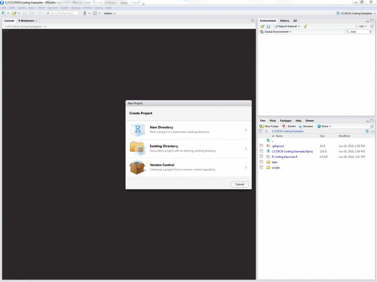
For the sake of these exercises (and for good file management practice), we will expect data files to be kept in “/name_of_your_directory/data”, and scripts to be kept in “/name_of_your_directory/scripts”. Once you have a new RStudio project inside a working directory created especially for this tutorial, you can add a blank R script (in RStudio, select File>New File> R Script) to your /scripts folder, into which you can copy and paste code from these exercises.
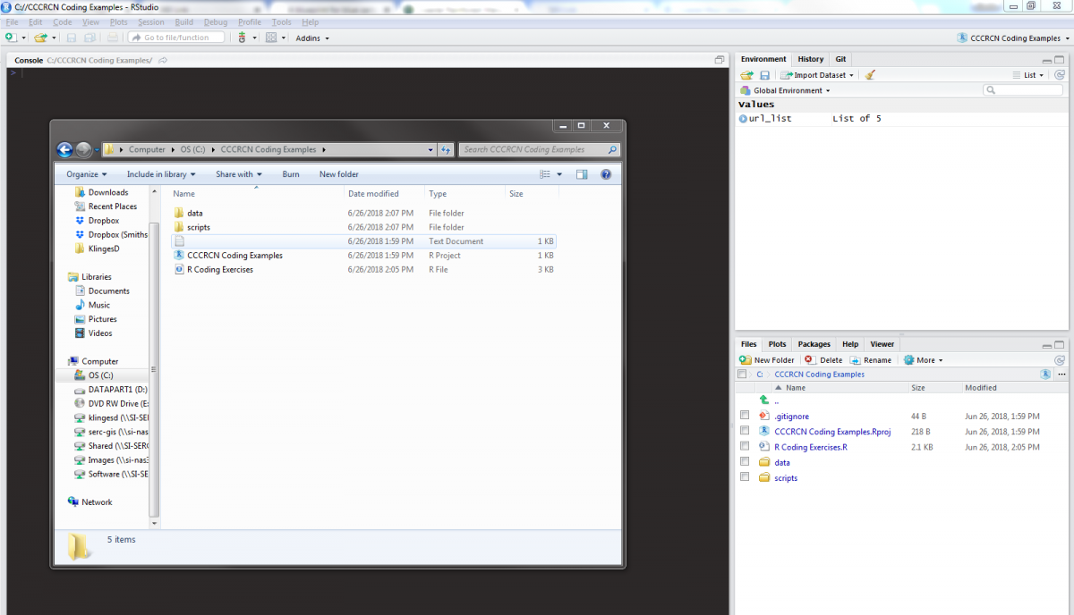
Although base R has many functions built-in, there are plenty of operations that are most effectively done by use of external packages. The following lines will install tidyverse and all other packages necessary for these exercises:
# Install packages
install.packages('tidyverse')
install.packages('RCurl')
install.packages('ggmap')
install.packages('rgdal')
We will use data from the CCRCN Soil Carbon Data Release (v1), which includes metadata on soil cores, the extent of human impact on core sites, field and lab methods, vegetation taxonomy, and soil carbon data. You can download the data files to your computer by clicking the links from the data release DOI, or download them manually using the following script:
(note: the following code will only work if you have created the appropriate folders, as described above)
# Load RCurl, a package used to download files from a URL
library(RCurl)

# Create a list of the URLs for each data file
url_list <- list(
    "https://repository.si.edu/bitstream/handle/10088/35684/V1_Holmquist_2018_core_data.csv?sequence=7&isAllowed=y",
    "https://repository.si.edu/bitstream/handle/10088/35684/V1_Holmquist_2018_depth_series_data.csv?sequence=8&isAllowed=y",
    "https://repository.si.edu/bitstream/handle/10088/35684/V1_Holmquist_2018_impact_data.csv?sequence=9&isAllowed=y",
    "https://repository.si.edu/bitstream/handle/10088/35684/V1_Holmquist_2018_methods_data.csv?sequence=10&isAllowed=y",
    "https://repository.si.edu/bitstream/handle/10088/35684/V1_Holmquist_2018_species_data.csv?sequence=11&isAllowed=y"
)

# Apply a function, which downloads each of the data files, over url_list
lapply(url_list, function(x) {
  # Extract the file name from each URL
  filename <- as.character(x)
  filename <- substring(filename, 56)
  filename <- gsub("\\..*","", filename)
  # Now download the file into the "data" folder
  download.file(x, paste0(getwd(), "/data/", filename, ".csv"))
})
Whether you used the links on the DOI or used the script, the data files should be downloaded into the /data folder of your working directory. Now let’s load them into our R project in RStudio and look at the column headers. We will use the tidyverse method of loading csv files with read_csv(), which automatically converts data frames into tibbles.
# Load tidyverse packages
library(tidyverse)
# Load data
core_data <- read_csv("data/V1_Holmquist_2018_core_data.csv")
impact_data <- read_csv("data/V1_Holmquist_2018_impact_data.csv")
methods_data <- read_csv("data/V1_Holmquist_2018_methods_data.csv")
species_data <- read_csv("data/V1_Holmquist_2018_species_data.csv")
depthseries_data <- read_csv("data/V1_Holmquist_2018_depth_series_data.csv")
Tibbles are the tidyverse-preferred version of data frames, with superior display options and a simpler design. There are a variety of methods to quickly view our tibbles, such as the depthseries_data tibble:
# Display data
glimpse(depthseries_data) # View all column headers and a sample of observations
## Observations: 16,976
## Variables: 8
## $ study_id                <chr> "Boyd_2012", "Boyd_2012", "Boyd_2012",...
## $ core_id                 <chr> "BBRC_1", "BBRC_1", "BBRC_1", "BBRC_1"...
## $ depth_min               <int> 0, 4, 8, 12, 16, 20, 24, 28, 32, 36, 4...
## $ depth_max               <int> 2, 6, 10, 14, 18, 22, 26, 30, 34, 38, ...
## $ dry_bulk_density        <dbl> 0.28, 0.41, 0.40, 0.48, 0.54, 0.59, 0....
## $ fraction_organic_matter <dbl> 0.28, 0.23, 0.27, 0.20, 0.18, 0.16, 0....
## $ fraction_carbon         <dbl> NA, NA, NA, NA, NA, NA, NA, NA, NA, NA...
## $ fraction_carbon_type    <chr> NA, NA, NA, NA, NA, NA, NA, NA, NA, NA...
head(depthseries_data) # View the first six observations of the dataset
## # A tibble: 6 x 8
##   study_id  core_id depth_min depth_max dry_bulk_density fraction_organic~
##   <chr>     <chr>       <int>     <int>            <dbl>             <dbl>
## 1 Boyd_2012 BBRC_1          0         2             0.28              0.28
## 2 Boyd_2012 BBRC_1          4         6             0.41              0.23
## 3 Boyd_2012 BBRC_1          8        10             0.4               0.27
## 4 Boyd_2012 BBRC_1         12        14             0.48              0.2
## 5 Boyd_2012 BBRC_1         16        18             0.54              0.18
## 6 Boyd_2012 BBRC_1         20        22             0.59              0.16
## # ... with 2 more variables: fraction_carbon <dbl>,
## #   fraction_carbon_type <chr>
tail(depthseries_data) # View the last six observations of the dataset
## # A tibble: 6 x 8
##   study_id   core_id depth_min depth_max dry_bulk_density fraction_organi~
##   <chr>      <chr>       <int>     <int>            <dbl>            <dbl>
## 1 Windham_M~ GL              0         2             1.67          0.0545
## 2 Windham_M~ GL              8        10             1.92          0.00906
## 3 Windham_M~ HH              0         2             1.66          0.0270
## 4 Windham_M~ HH              8        10             1.34          0.0256
## 5 Windham_M~ HL              0         2             1.40          0.0579
## 6 Windham_M~ HL              8        10             1.87          0.00947
## # ... with 2 more variables: fraction_carbon <dbl>,
## #   fraction_carbon_type <chr>
names(depthseries_data) # View the names of all column headers
## [1] "study_id"                "core_id"
## [3] "depth_min"               "depth_max"
## [5] "dry_bulk_density"        "fraction_organic_matter"
## [7] "fraction_carbon"         "fraction_carbon_type"
The ability to quickly view your data in different ways will inform what manipulations are needed to be performed. Besides these commands, you can also click on an object in the “Environment” tab of RStudio:

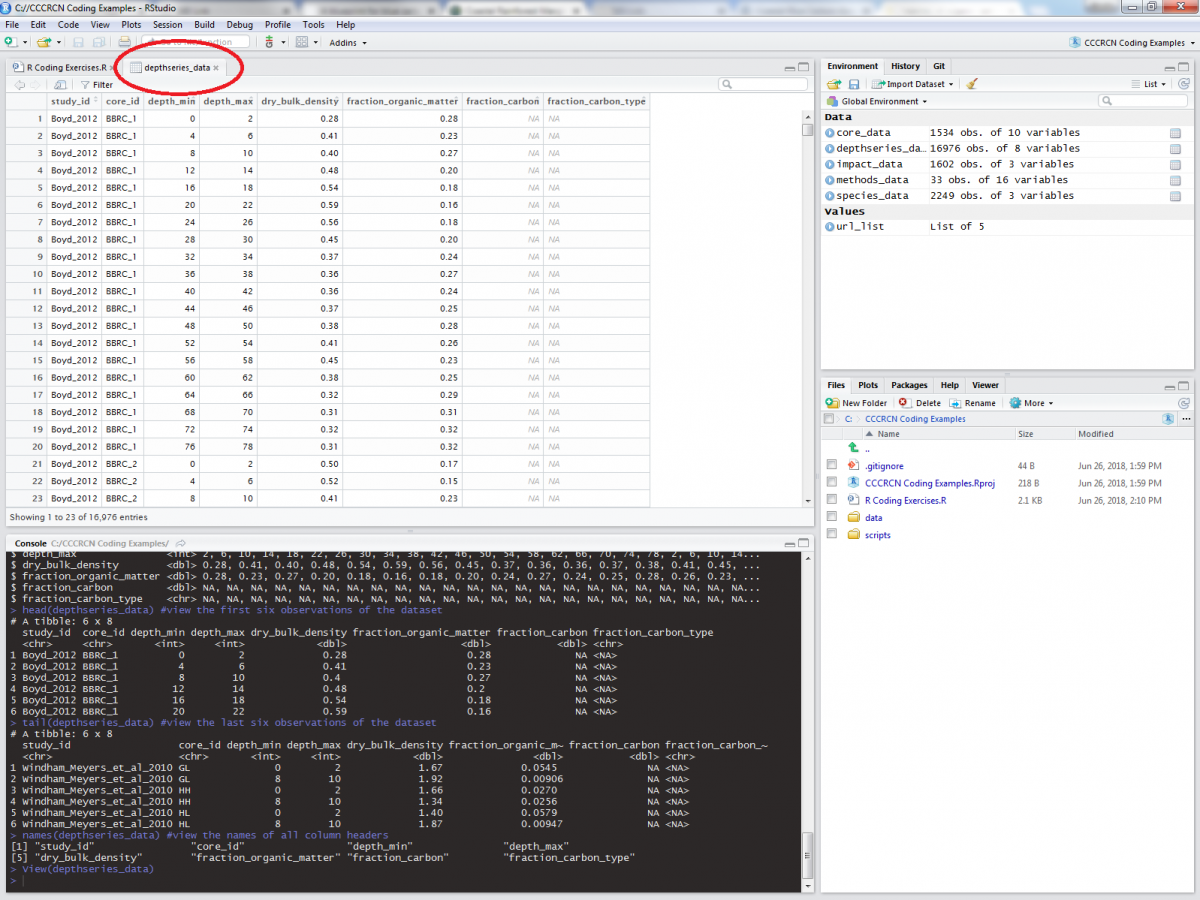
Let’s take a quick look at the columns provided in the depthseries_data tibble (this metadata can be found online here, which is also linked on the dataset DOI):
| Column header | Meaning |
|---|---|
| study_id | Unique identified for the study made up of the first author’s family name, as well as the second author’s or ‘et al.’ |
| core_id | Unique identifier assiged to a core. |
| depth_min | Minimum depth of a sampling increment. |
| depth_max | Maximum depth of a sampling increment. |
| dry_bulk_density | Dry mass per unit volume of a soil sample. |
| fraction_organic_matter | Mass of organic matter relative to sample dry mass. |
| fraction_carbon | Mass of carbon relative to sample dry mass. |
| fraction_carbon_type | Code assigned to specify the type of measurement fraction_carbon represents. |
A lot of interesting types of data to work with here. But we can change what is included as well, by adding and removing columns.
Add and Remove Columns
Add and Remove Columns
To manipulate our datasets, we are going to use the dplyr package, a component of the tidyverse (and so dplyr is automatically installed with tidyverse). dplyr is a package dedicated to data wrangling, and will come in great use to us.
We will be performing many modifications to our datasets in these exercises, but to leave ourselves a trail of breadcrumbs back to the original data, we will want to create new datasets instead of permanently modifying the original tibbles. For this, we will create a new object for each modification. Assigning a value to an object is an integral component of R and many coding practices:
# create an object
x <- 3
x
## [1] 3
This will come in handy when we want to modify one of our datasets. Sometimes the data we are seeking is not included in the original data, but is a product of existing columns. For instance, it may be useful to calculate organic matter density by multiplying dry bulk density (g * cm-3) by the fraction of soil that is organic matter (fraction). To do this, we can use the mutate() operation:
# calculate organic matter density
depthseries_data_with_organic_matter_density <- mutate(depthseries_data,
       organic_matter_density = dry_bulk_density * fraction_organic_matter)

head(depthseries_data_with_organic_matter_density)
## # A tibble: 6 x 9
##   study_id  core_id depth_min depth_max dry_bulk_density fraction_organic~
##   <chr>     <chr>       <int>     <int>            <dbl>             <dbl>
## 1 Boyd_2012 BBRC_1          0         2             0.28              0.28
## 2 Boyd_2012 BBRC_1          4         6             0.41              0.23
## 3 Boyd_2012 BBRC_1          8        10             0.4               0.27
## 4 Boyd_2012 BBRC_1         12        14             0.48              0.2
## 5 Boyd_2012 BBRC_1         16        18             0.54              0.18
## 6 Boyd_2012 BBRC_1         20        22             0.59              0.16
## # ... with 3 more variables: fraction_carbon <dbl>,
## #   fraction_carbon_type <chr>, organic_matter_density <dbl>
Notice that we have 9 columns instead of 8, as we did before? That's because we've successfully added organic matter density. We now have more columns than we can easily display in the console, which is one (of many) reasons that you may want to manipulate how many, and which, columns we choose to include. In our present case, we want to simplify our dataset to just a few columns. For this, we select() which columns we desire.
# Select just a handful of columns
depthseries_data_select <- select(depthseries_data_with_organic_matter_density, # Define dataset
                                  core_id, depth_min, depth_max, organic_matter_density) # Chosen columns

head(depthseries_data_select)
## # A tibble: 6 x 4
##   core_id depth_min depth_max organic_matter_density
##   <chr>       <int>     <int>                  <dbl>
## 1 BBRC_1          0         2                 0.0784
## 2 BBRC_1          4         6                 0.0943
## 3 BBRC_1          8        10                 0.108
## 4 BBRC_1         12        14                 0.096
## 5 BBRC_1         16        18                 0.0972
## 6 BBRC_1         20        22                 0.0944
This display looks much better. We can also perform both the mutate and select operations in the same command by using dplyr’s pipe notation, %>%. The pipe notation is useful for a few reasons. First, you can call many operations in quick succession on the same dataset. It makes for cleaner, more readable code: we can easily display each operation on a new line, and we move the dataset from the first argument in each of the operations to outside and in front of the function. You can say to yourself as you type %>%, "I'm putting the dataset on the left through the function below". Don't worry about being judged while talking to yourself, just tell people you're learning how to code in R and they will forgive a lot of strange behavior.
# Calculate organic matter density, then remove all non-critical columns
depthseries_data_select <- depthseries_data %>% # Define dataset
# Separate operations with "%>%"
  mutate(organic_matter_density = dry_bulk_density * fraction_organic_matter) %>%
# Even though we just created the organic_matter_density column,
# we can immediately use it in the select() operation
  select(core_id, depth_min, depth_max, organic_matter_density)

head(depthseries_data_select)
## # A tibble: 6 x 4
##   core_id depth_min depth_max organic_matter_density
##   <chr>       <int>     <int>                  <dbl>
## 1 BBRC_1          0         2                 0.0784
## 2 BBRC_1          4         6                 0.0943
## 3 BBRC_1          8        10                 0.108
## 4 BBRC_1         12        14                 0.096
## 5 BBRC_1         16        18                 0.0972
## 6 BBRC_1         20        22                 0.0944
Last Page Return to Top Next Page
Organize Observations
Organize Observations
Sorting rows by particular values of a column is a common intermediary step for analysis and plot generation, and also is helpful to quickly view your data in different arrangements. One of the methods we can use to do so is with group_by(). This operation will place observations that have the same value of a given column ("core_id") next to each other:
# Sort data with group_by
depthseries_data_grouped <- group_by(depthseries_data_select, core_id)
head(depthseries_data_grouped)
## # A tibble: 6 x 4
##   core_id depth_min depth_max organic_matter_density
##   <chr>       <int>     <int>                  <dbl>
## 1 BBRC_1          0         2                 0.0784
## 2 BBRC_1          4         6                 0.0943
## 3 BBRC_1          8        10                 0.108
## 4 BBRC_1         12        14                 0.096
## 5 BBRC_1         16        18                 0.0972
## 6 BBRC_1         20        22                 0.0944
tail(depthseries_data_grouped)
## # A tibble: 6 x 4
##   core_id depth_min depth_max organic_matter_density
##   <chr>       <int>     <int>                  <dbl>
## 1 GL              0         2                 0.0910
## 2 GL              8        10                 0.0174
## 3 HH              0         2                 0.0447
## 4 HH              8        10                 0.0344
## 5 HL              0         2                 0.0811
## 6 HL              8        10                 0.0177
It didn't seem like it did anything, did it? The rows are now arranged by core_id (BBRC_1,BBRC_2, NCBD_1, etc.), much in the same manner that they originally were. That's OK. the group_by operation isn't really useful on it's own, but can be very powerful when paired with other operations. Here's one: if you want to condense your data to one row according to one attribute, you can do so with the summarize() operation.
# What is the average organic matter density of all observations
depthseries_data_avg_organic_matter_density <- summarize(depthseries_data_select, # Define dataset
  organic_matter_density_avg = mean(organic_matter_density, # New column that has one entry,
                                                            # the mean organic matter density
  na.rm = TRUE)) # Remove NA values before summarizing
depthseries_data_avg_organic_matter_density
## # A tibble: 1 x 1
##   organic_matter_density_avg
##                        <dbl>
## 1                     0.0679
This is the average organic matter density for all of our data. Now what if we wanted to calculate the average organic matter density for each core? Although group_by() and summarize() aren't that interesting by themselves, they are really effective when used in sequence:
# What is the average organic matter density of each core, for all cores
depthseries_data_avg_OMD_by_core <- depthseries_data_select %>%
  group_by(core_id) %>%
  summarize(organic_matter_density_avg = mean(organic_matter_density, na.rm = TRUE))
depthseries_data_avg_OMD_by_core
## # A tibble: 1,534 x 2
##    core_id                     organic_matter_density_avg
##    <chr>                                            <dbl>
##  1 AH                                              0.109
##  2 AL                                              0.0930
##  3 Alley_Pond                                      0.0734
##  4 Altamaha_River_Site_7_Levee                   NaN
##  5 Altamaha_River_Site_7_Plain                   NaN
##  6 Altamaha_River_Site_8_Levee                   NaN
##  7 Altamaha_River_Site_8_Plain                   NaN
##  8 Altamaha_River_Site_9_Levee                   NaN
##  9 Altamaha_River_Site_9_Plain                   NaN
## 10 AND                                             0.0690
## # ... with 1,524 more rows
Using these two operations with the %>% notation, we were able to find the mean organic matter density for each of the cores in our dataset.
Last Page Return to Top Next Page
Plot a Histogram
Plot a Histogram
Now we will use these skills in unison to create a plot of our data. For this, we will use the ggplot2 package, also part of the tidyverse. The template for visualizations generated by ggplot involve base inputs through the ggplot() operation, followed by aesthetics added with aes() and layouts generated with theme(). There is a vast array of kinds of plots we can create in R through ggplot, but we will start with a simple histogram of carbon density.
First, we must calculate carbon density. Some of the studies in our data calculated the fraction mass of the sample that is carbon, which is needed to calculate carbon density. However, not all studies included this calculation. We will need to estimate the fraction carbon from the fraction organic matter, using the quadratic formula derived by Holmquist et al (2018).
In order to accomplish this, we will create a function that estimates the fraction carbon using the Holmquist et al (2018) equation. Then, we will write an if-else statement: if a logical statement is TRUE, then an action is performed; if the statement is FALSE, a different action is performed:
# This function estimates fraction carbon as a function of fraction organic matter
estimate_fraction_carbon <- function(fraction_organic_matter) {

# Use the quadratic relationship published by Holmquist et al. 2018 to derive the fraction of carbon from the
# fraction of organic matter

  fraction_carbon <- (0.014) * (fraction_organic_matter ^ 2) + (0.421 * fraction_organic_matter) + (0.008)
  if (fraction_carbon < 0) {
    fraction_carbon <- 0 # Replace negative values with 0
  }
  return(fraction_carbon) # The product of the function is the estimated fraction carbon value
}

depthseries_data_with_carbon_density <- depthseries_data %>% # For each row in depthseries_data...
  mutate(carbon_density =
    ifelse(! is.na(fraction_carbon), # IF the value for fraction_carbon is not NA....
# Then a new variable, carbon density, equals fraction carbon * dry bulk density....
      (fraction_carbon * dry_bulk_density),
# ELSE, carbon density is estimated using our function
      (estimate_fraction_carbon(fraction_organic_matter) * dry_bulk_density)
    )
  )

glimpse(depthseries_data_with_carbon_density)
## Observations: 16,976
## Variables: 9
## $ study_id                <chr> "Boyd_2012", "Boyd_2012", "Boyd_2012",...
## $ core_id                 <chr> "BBRC_1", "BBRC_1", "BBRC_1", "BBRC_1"...
## $ depth_min               <int> 0, 4, 8, 12, 16, 20, 24, 28, 32, 36, 4...
## $ depth_max               <int> 2, 6, 10, 14, 18, 22, 26, 30, 34, 38, ...
## $ dry_bulk_density        <dbl> 0.28, 0.41, 0.40, 0.48, 0.54, 0.59, 0....
## $ fraction_organic_matter <dbl> 0.28, 0.23, 0.27, 0.20, 0.18, 0.16, 0....
## $ fraction_carbon         <dbl> NA, NA, NA, NA, NA, NA, NA, NA, NA, NA...
## $ fraction_carbon_type    <chr> NA, NA, NA, NA, NA, NA, NA, NA, NA, NA...
## $ carbon_density          <dbl> 0.03555373, 0.04328395, 0.04907624, 0....
All of our newly calculated carbon_density data is within a new column of the same name. Let’s compile this information into a visual using ggplot. For displaying the distribution of carbon density, a histogram will do.
# Create a histogram of carbon density
histo <- ggplot(data = depthseries_data_with_carbon_density, # Define dataset
       aes(carbon_density)) + # Define which data is displayed
       geom_histogram(bins = 100) # Determine bin width, and therefore number of bins displayed

histo
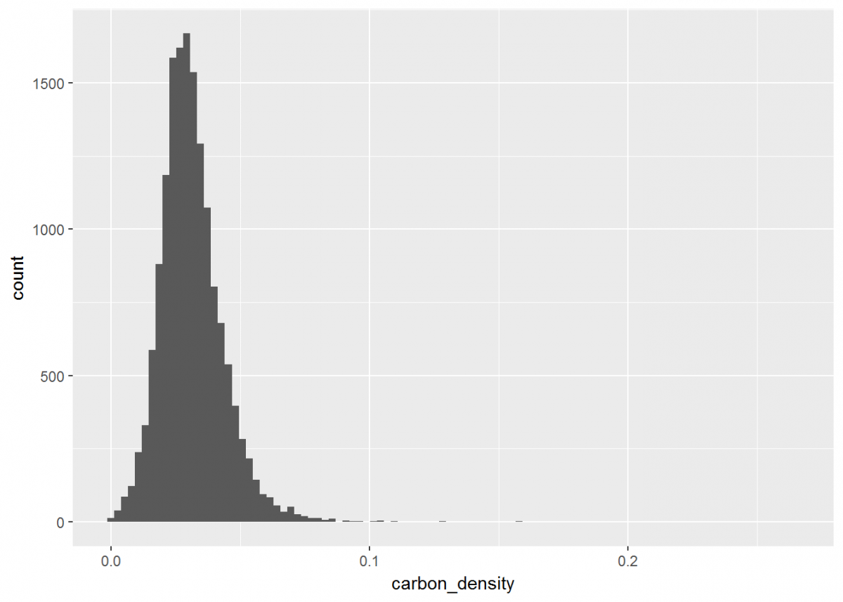
Notice how ggplot has its own notation that is different from dplyr, but the two packages are similar in that you can stack operations one after another. While dplyr uses the %>% notation, ggplot's syntax is a plus sign +. Also, you likely received a warning that rows containing non-finite values were removed. This is because ggplot recognized that some of our data was NA, and did not plot these entries.
Our plot could look a little better if the limit of the x-axis was reduced to fit the distribution…and let’s change the theme background and plot labels while we're at it.
# Update our histogram
histo <- histo + # Load the plot that we've already made
         xlim(0, 0.15) + # Change x-axis limit to better fit the data
         theme_classic() + # Change the plot theme
         ggtitle("Distribution of Carbon Density of CONUS") + # Give the plot a title (CONUS = contiguous US)
         xlab("Carbon Density") + # Change x axis title
         ylab("Number of Observations") # Change y axis title
histo
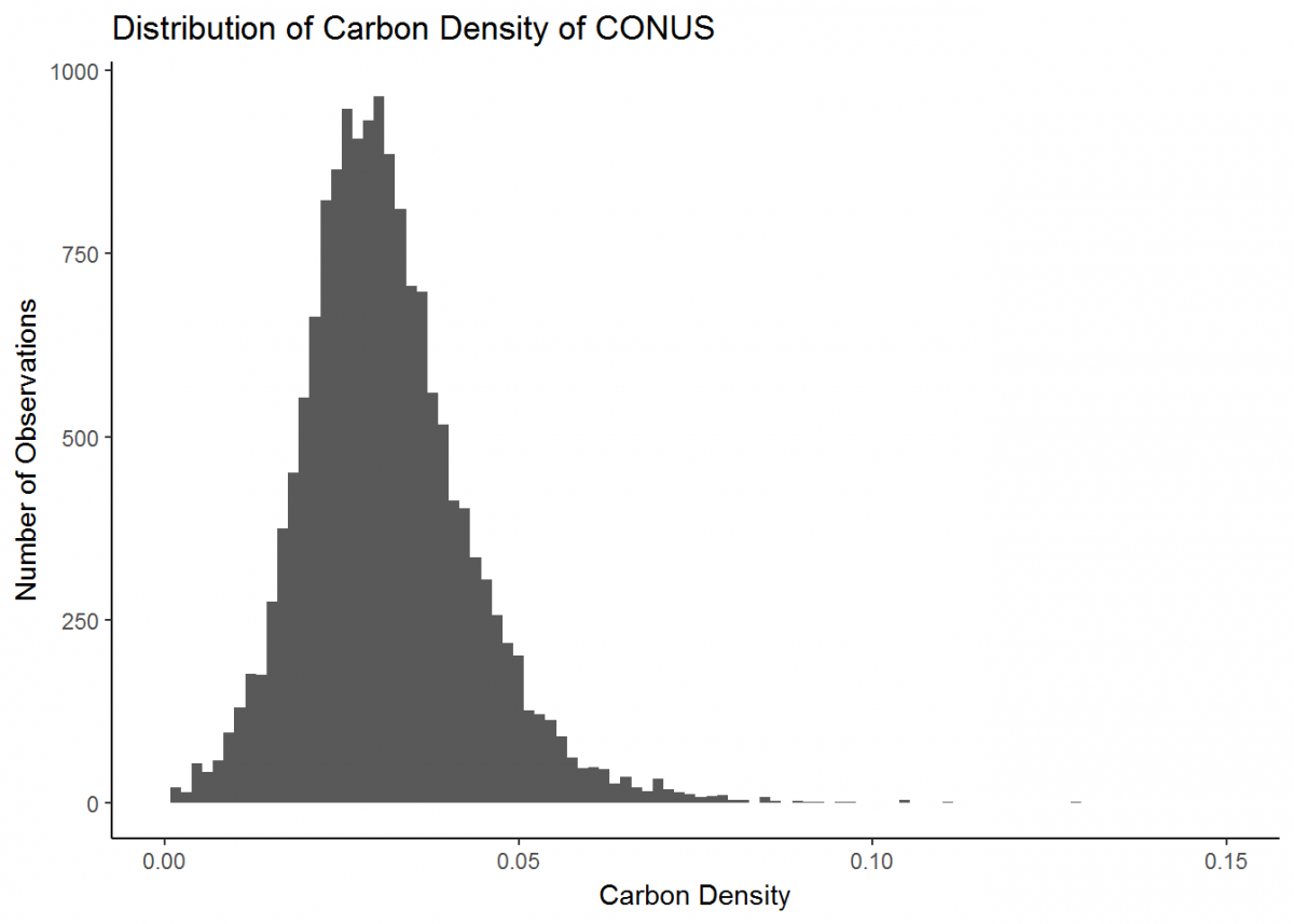
Great, much better. This is a basic plot of just one type of data. However, there is much more you can do with the functionality of ggplot (the ggplot cheatsheet provides some quick overview), and soon we will develop more intricate plots with multiple data types. But first, we’ll learn a couple new skills.
Last Page Return to Top Next Page
Join and Filter Data
Join and Filter Data
We will now learn a few more dplyr commands that will lead us to developing a map of soil cores.
Sometimes it might be useful to combine the contents of one dataset with a different dataset; say, to look at how the fraction of organic carbon varies with geographic location. There is a suite of commands in dplyr that can do so in different fashions, all of which are in “_join()" format. For our purposes, left_join() works:
# left_join pulls rows in the 2nd given dataset that match existing rows in the first given dataset via a common
# key (e.g. core_id)
core_depth_data <- left_join(core_data, depthseries_data, by = NULL)
## Joining, by = c("study_id", "core_id")
head(core_depth_data)
## # A tibble: 6 x 16
##   study_id  core_id core_latitude core_longitude position_code core_elevation salinity_code
##   <chr>     <chr>           <dbl>          <dbl> <chr>                  <dbl> <chr>
## 1 Boyd_2012 BBRC_1           39.4          -75.7 a1                        NA Bra
## 2 Boyd_2012 BBRC_1           39.4          -75.7 a1                        NA Bra
## 3 Boyd_2012 BBRC_1           39.4          -75.7 a1                        NA Bra
## 4 Boyd_2012 BBRC_1           39.4          -75.7 a1                        NA Bra
## 5 Boyd_2012 BBRC_1           39.4          -75.7 a1                        NA Bra
## 6 Boyd_2012 BBRC_1           39.4          -75.7 a1                        NA Bra
## # ... with 9 more variables: vegetation_code <chr>, inundation_class <chr>, core_length_flag <chr>,
## #   depth_min <int>, depth_max <int>, dry_bulk_density <dbl>, fraction_organic_matter <dbl>,
## #   fraction_carbon <dbl>, fraction_carbon_type <chr>
Sometimes two datasets you wish to join have different names for the same variable (e.g., “name” and “Name”, or “temp” and “C”). If this is the case, you can specify which variables you wish to join together using the “by” argument [ex: left_join(...by = c("name" = "Name"))]. Because our data has uniform terminology and syntax, we didn’t need to do this, so the “by” argument is left as NULL above [the default value for “by” in all _join() commands is NULL, but we included it to illustrate the point].
Now that our core data and depth series data are both in the same tibble, we can perform new operations on them. To explore particular parts of the data, we often are interested in subsetting to rows with a common characteristic. The filter() operation allows for this to be done easily.
# Filter to just cores with coordinates from a high quality source
core_data_HQ_coord <- filter(core_data, position_code == 'a1')
# We can use logical symbols in our filter operation
core_data_HQ_coord <- filter(core_data, position_code == 'a1' | position_code == 'a2')
# And, we can filter by more than one criterion
core_data_HQ_coord_estuarine <- filter(core_data, position_code == 'a1' | position_code == 'a2',
salinity_code == 'Est')

head(core_data_HQ_coord_estuarine)
## # A tibble: 6 x 10
##   study_id          core_id core_latitude core_longitude position_code core_elevation salinity_code
##   <chr>             <chr>           <dbl>          <dbl> <chr>                  <dbl> <chr>
## 1 Crooks_et_al_2013 MA_A             48.0          -122. a1                      6.41 Est
## 2 Crooks_et_al_2013 MA_B             48.0          -122. a1                      6.54 Est
## 3 Crooks_et_al_2013 NE_A             48.0          -122. a1                      7.86 Est
## 4 Crooks_et_al_2013 NE_B             48.0          -122. a1                     NA    Est
## 5 Crooks_et_al_2013 QM_A             48.0          -122. a1                      6.12 Est
## 6 Crooks_et_al_2013 QM_B             48.0          -122. a1                      5.99 Est
## # ... with 3 more variables: vegetation_code <chr>, inundation_class <chr>, core_length_flag <chr>
This allows us to select observations that fulfill particular requirements; in this case, we wanted only cores with high-quality georeferencing, and therefore with ‘a1’ as its position_code.
Last Page Return to Top Next Page
Plot Maps
Plot Maps
Let’s finish by creating more visuals; this time, a series of maps. The core_data tibble includes longitude and latitude of each soil core, so we can use those coordinates to plot where the cores were taken in geographical space:
    # Plot cores on a lat/long coordinate plane
    map <- ggplot() +
    geom_point(data = core_data, aes(x = core_longitude, y = core_latitude)) + # Add coordinate data
    theme_bw() + # Change the plot theme
    ggtitle("Distribution of Sampled Cores across CONUS") + # Give the plot a title
    xlab("Longitude") + # Change x axis title
    ylab("Latitude") # Change y axis title
    map

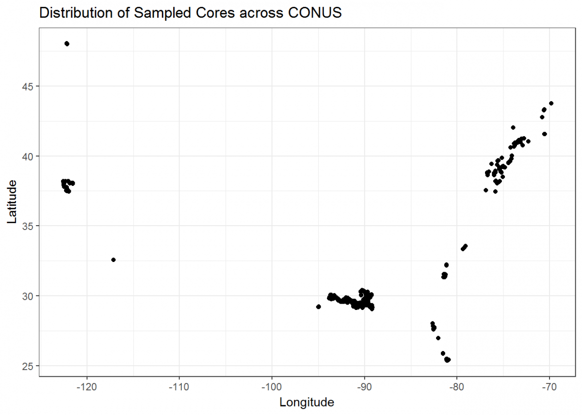
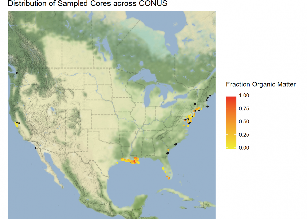
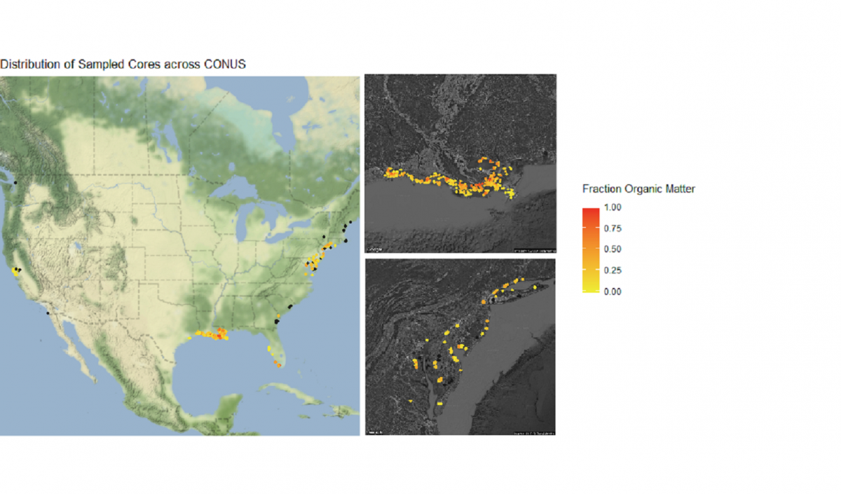
Not bad, but we can do more. Let’s plot a coordinate display of our cores overlayed on top of a map of the conterminous US, and display cores by a color gradient corresponding to the fraction of organic matter. We’ll use many of the operations that we learned in this tutorial all in sequence.
We’re also going to integrate a few packages that help with processing and displaying spatial data, rgdal and ggmap.
    # Load new packages
    devtools::install_github("dkahle/ggmap") # As of time of writing, this is a package that receives frequent
    # updates. So it's good to install from GitHub
    library(ggmap)
    library(rgdal)

    # Join core_data and depthseries_data
    core_depth_data <- left_join(core_data, depthseries_data, by = NULL)

    # Select coordinate data from core_data and redefine into new dataset
    core_coordinates <- select(core_depth_data, core_longitude, core_latitude, fraction_organic_matter)


    # Add Google Maps image of CONUS to plot
    CONUS_map <- get_map(location = c(lon = -96.5795, lat = 39.8283), # center map on CONUS
    color = "color",
    source = "google",
    maptype = "terrain-background",
    zoom = 4) # set the zoom to include all data

    # Add the CONUS_map with axes set as Longitude and Latitude
    ggmap(CONUS_map,
    extent = "device",
    xlab = "Longitude",
    ylab = "Latitude") +

    # Add core lat/long coordinates as points, colored by fraction organic matter
    geom_point(data = core_coordinates, aes(x = core_longitude, y = core_latitude, color =
    fraction_organic_matter), alpha = 1, size = 1) +
    scale_color_gradientn("Fraction Organic Matter\n",
    colors = c("#EFEC35", "#E82323"), na.value = "#1a1a1a") + # Provide ggplot2 with color gradient
    ggtitle("Distribution of Sampled Cores across CONUS") + # Give the plot a title
    xlab("Longitude") + # Change x axis title
    ylab("Latitude") # Change y axis title

    # Filter to specific regions for map insets

    # Add inset of Coastal Louisiana
    LA_map <- get_map(location = c(lon = -91.0795, lat = 30.2283),
    color = "bw",
    source = "google",
    maptype = "satellite",
    zoom = 7)

    # Add the LA_map with axes set as Longitude and Latitude
    ggmap(LA_map,
    extent = "device",
    xlab = "Longitude",
    ylab = "Latitude") +

    # Add core lat/long coordinates as points, colored by fraction organic matter
    geom_point(data = core_coordinates, aes(x = core_longitude, y = core_latitude, color =
    fraction_organic_matter), alpha = 1, size = 2) +
    scale_color_gradientn("Fraction Organic Matter\n",
    colors = c("#EFEC35", "#E82323"), na.value = "#1a1a1a") # Provide ggplot2 with color gradient

    # Add inset of Mid-Atlantic Seaboard
    mid_Atlantic_map <- get_map(location = c(lon = -75.095, lat = 39.2283),
    color = "bw",
    source = "google",
    maptype = "satellite",
    zoom = 7)

    # Add the mid_Atlantic_map with axes set as Longitude and Latitude
    ggmap(mid_Atlantic_map,
    extent = "device",
    xlab = "Longitude",
    ylab = "Latitude") +

    # Add core lat/long coordinates as points, colored by fraction organic matter
    geom_point(data = core_coordinates, aes(x = core_longitude, y = core_latitude, color =
    fraction_organic_matter), alpha = 1, size = 3) +
    scale_color_gradientn("Fraction Organic Matter\n",
    colors = c("#EFEC35", "#E82323"), na.value = "#1a1a1a") # Provide ggplot2 with color gradient

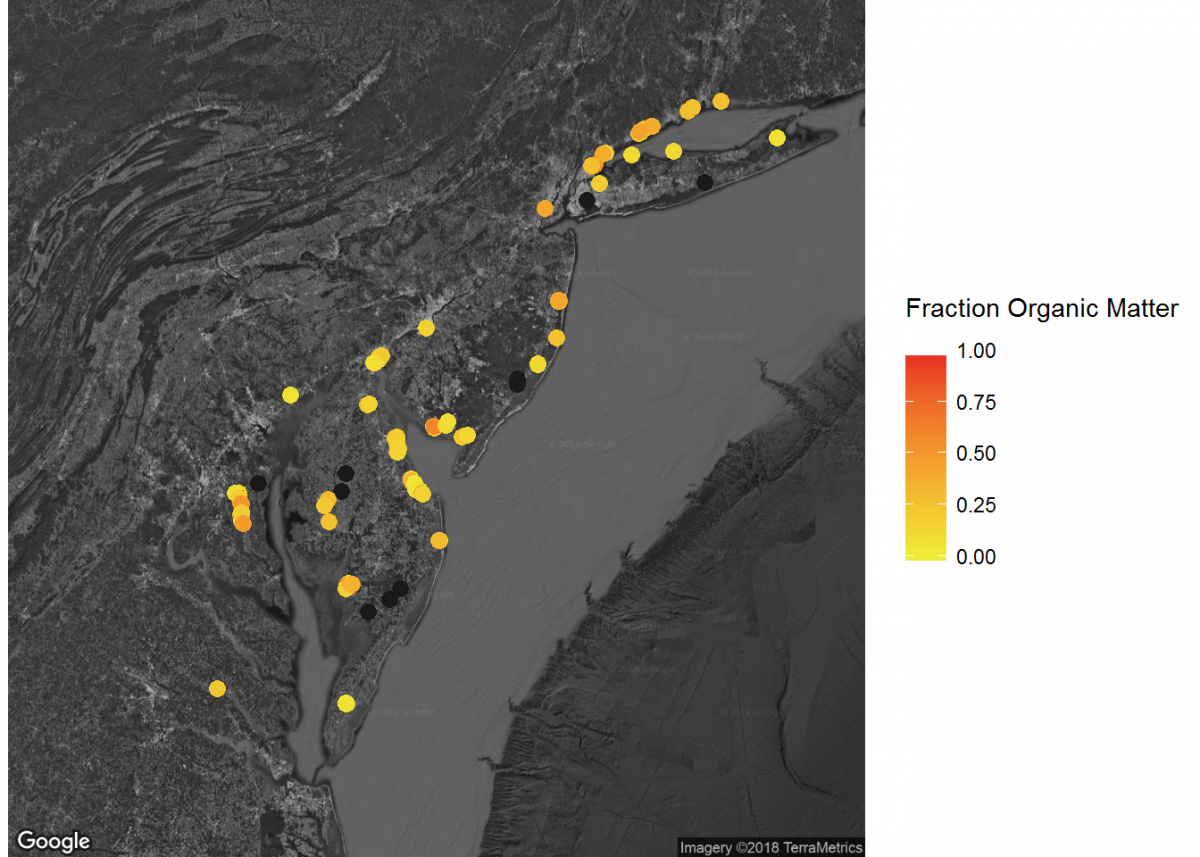
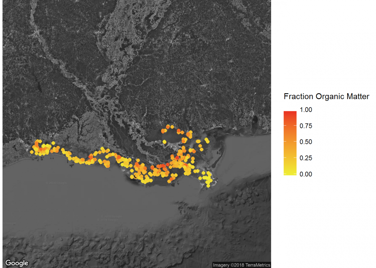
When combined, these maps can tell a lot about soil carbon across the contiguous United States.
Last Page Return to Top Next Page
Challenge Exercises
Challenge Exercises
Now is time to put what you learned to the test with some challenges. Below are a few tasks for you to conduct in order to practice the commands you just learned. Your challenge is to use what you know about mutate, group_by and summarize, filter, and plotting in ggplot to complete the following tasks. Struggle builds character, but if you need a hint or want to check your answer, click the corresponding Hint and Solution buttons below.
- Calculate organic matter density from bulk density and fraction organic matter. What is the average organic matter density in natural (impact_code = Nat) versus restored (impact_code = Res) sites?
First, We'll need to create a new column (organic matter density) that uses data from existing columns...sound familiar? Then, we'll need to combine data from two different data sets: depthseries and impact. Finally, we'll need to filter data to just the cores obtained from sites with the specified impact codes, and for each of these impact codes find the summary stat (mean) of our calculated column, organic matter density. We won't be able to correctly calculate our averages if there are any NA values for organic matter density, however. Give it a try!
# First, we'll need to calculate organic matter density. We did this earlier in the tutorial as well
depthseries_data_with_organic_matter_density <- depthseries_data %>%
mutate(organic_matter_density = dry_bulk_density * fraction_organic_matter)
# Now, we'll join together the depthseries and impact data
depthseries_with_omd_and_impact <- depthseries_data_with_organic_matter_density %>%
left_join(impact_data)
# We won't be able to summarize data if there are any NA values
depthseries_with_omd_and_impact <- depthseries_with_omd_and_impact %>%
filter(!is.na(organic_matter_density))

# Summarize for natural sites
depthseries_with_omd_and_impact %>%
filter(impact_code == "Nat") %>%
summarize(mean(organic_matter_density))

# Summarize for restored sites
depthseries_with_omd_and_impact %>%
filter(impact_code == "Res") %>%
summarize(mean(organic_matter_density))
# Organic matter density is slightly higher in natural sites than restored sites.
- Plot a histogram of carbon density from 0 to 5 cm.
We will need to first subset to just the data we want: the depth series observations from a depth less than or equal to 5 cm. To do so, we'll need to group depth series observations by what core they are from, and then filter to just those from our desired depths. You will probably want to create a new object from our selected data. Then it's just as simple as constructing a histogram plot of our selected data. Check out the ggplot2 cheat sheet to help with this: https://www.rstudio.com/wp-content/uploads/2015/03/ggplot2-cheatsheet.pdf
# Filter for just data collected at depths of 5 cm or less
depthseries_data_shallow <- depthseries_data_with_carbon_density %>%
filter(depth_max <= 5)
# Plot the data as a histogram
depth_weighted_average_plot <- ggplot(depthseries_data_shallow, aes(carbon_density)) +
geom_histogram(bins = 100)
depth_weighted_average_plot
- For each core with a maximum depth greater than or equal to 50 cm, calculate the average carbon density.
This is a tough one. Like the last challenge, we'll need to subset to just the cores we want. This time, we'll then need to acquire a summary stat for each core: the maximum value of the depth_max column. We want to filter to just cores that have such a value greater than or equal to 50...but we also have to make sure we retain ALL of the depth series observations for these long cores, including the observations at depths less than 50 cm. Once we have successfully accomplished this, we know the drill: calculate the average carbon density of the data grouped by each core.
# There are several methods by which you can narrow our selection of cores to just those that we want:
# Solution 1
depthseries_max_depths <- depthseries_data_with_carbon_density %>%
group_by(core_id) %>%
summarize(max_depth = max(depth_max))
# Create a new column, which contains the maximum depth sampled in each core
depthseries_data_long_cores <- depthseries_data_with_carbon_density %>%
left_join(depthseries_max_depths) %>%
# Join our depthseries data to the dataset that contains maximum depths
filter(max_depth >= 50)  # Select for only cores longer than 50 cm

# Another method is even more simple:
# Solution 2
depthseries_data_long_cores <- depthseries_data_with_carbon_density %>%
group_by(core_id) %>%
filter(max(depth_max) >= 50)

# Now calculate average carbon density
long_cores_average_carbon_density <- depthseries_data_long_cores %>%
group_by(core_id) %>%
summarize(mean(carbon_density))

long_cores_average_carbon_density
Additional Resources
There is loads more that can be accomplished with our data using the tidyverse. But it’s easy to get overwhelmed by the many operations available, so the RStudio cheat sheets are immensely helpful:
We realize that learning a new coding language is a lot to take on: it’s a marathon, not a sprint. To help with that process, here are some additional resources that offer an introduction to R and RStudio:
Now you’re ready to take advantage of the full potential of your data!
Tell us how we did:
Any thoughts on these tutorials? Send them along to CoastalCarbon@si.edu, we appreciate the feedback.