Data Manipulation in R: Introduction
Questions about this tutorial? Contact David Klinges at KlingesD@si.edu or James Holmquist at HolmquistJ@si.edu
The CCRCN aspires to make data accessible and easy to manipulate. These exercises are directed towards an audience that is already a beginner R user and has worked with RStudio, but is open to a new toolset. If you’re not comfortable with R yet, take a look at the Resources listed at the bottom of the last page (Challenge Exercises). Here, we will manipulate coastal carbon data using the tools available in the tidyverse. The tidyverse suite of packages is designed for data science, and all adheres to similar grammar and data structure. In order to both most efficiently use data curated by the CCRCN– and also to be familiar with some of the more flexible and popular data science tools used in the sciences– tidyverse is important to learn.
First, we are going to prep our workspace, by setting our directory and loading the data. Next, we will demonstrate how to modify the columns of a dataset to fit one’s needs, and then we will show how to group and summarize observations by certain attributes. From there, we will build a simple visualization of our data. We’ll then learn a few new skills, build maps from our data, and finally test our new abilities with some challenges.
Prepare workspace
We start by opening RStudio and creating a new project. RStudio projects work through a selected working directory, where all pertinent files are located.
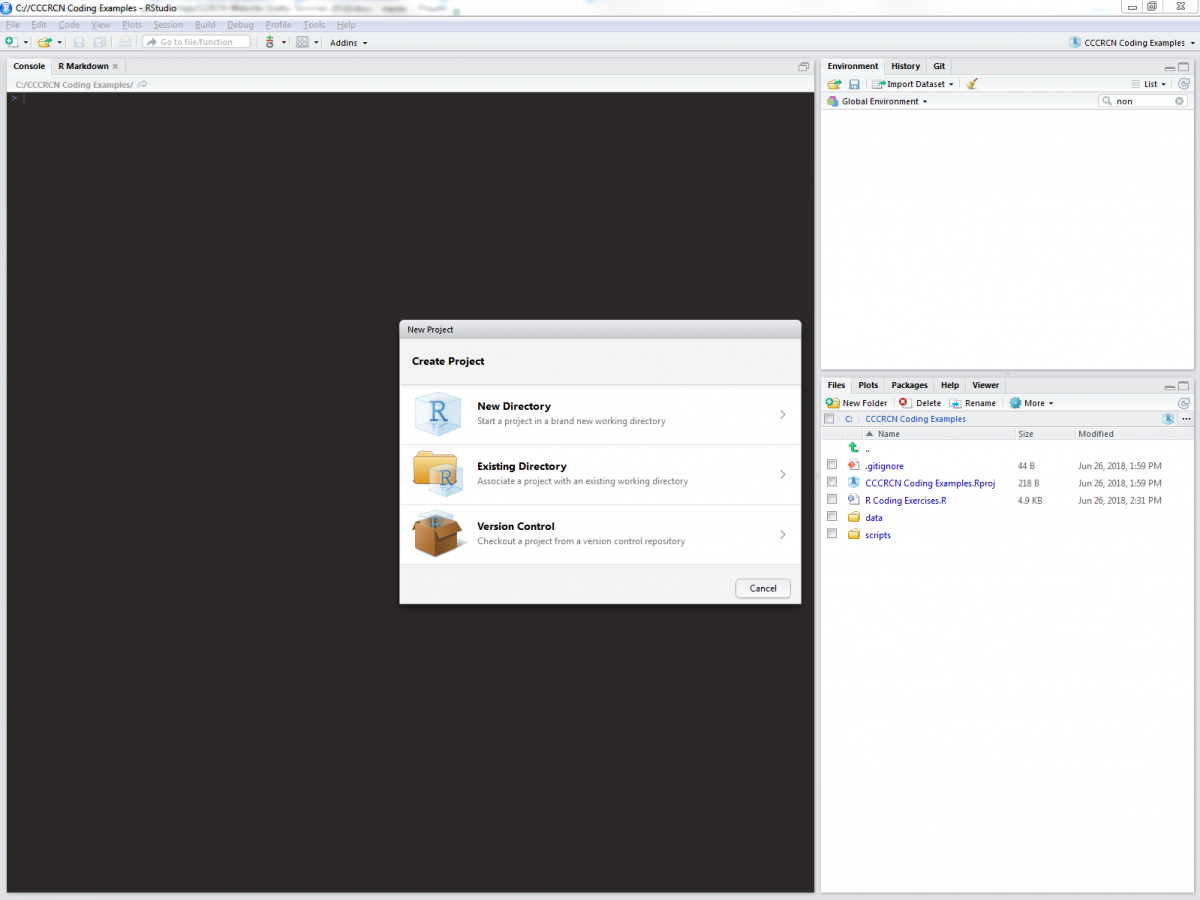
For the sake of these exercises (and for good file management practice), we will expect data files to be kept in “/name_of_your_directory/data”, and scripts to be kept in “/name_of_your_directory/scripts”. Once you have a new RStudio project inside a working directory created especially for this tutorial, you can add a blank R script (in RStudio, select File>New File> R Script) to your /scripts folder, into which you can copy and paste code from these exercises.
Although base R has many functions built-in, there are plenty of operations that are most effectively done by use of external packages. The following lines will install tidyverse and all other packages necessary for these exercises:
# Install packages
install.packages('tidyverse')
install.packages('RCurl')
install.packages('ggmap')
install.packages('rgdal')
We will use data from the CCRCN Soil Carbon Data Release (v1), which includes metadata on soil cores, the extent of human impact on core sites, field and lab methods, vegetation taxonomy, and soil carbon data. You can download the data files to your computer by clicking the links from the data release DOI, or download them manually using the following script:
(note: the following code will only work if you have created the appropriate folders, as described above)
# Load RCurl, a package used to download files from a URL
library(RCurl)

# Create a list of the URLs for each data file
url_list <- list(
    "https://repository.si.edu/bitstream/handle/10088/35684/V1_Holmquist_2018_core_data.csv?sequence=7&isAllowed=y",
    "https://repository.si.edu/bitstream/handle/10088/35684/V1_Holmquist_2018_depth_series_data.csv?sequence=8&isAllowed=y",
    "https://repository.si.edu/bitstream/handle/10088/35684/V1_Holmquist_2018_impact_data.csv?sequence=9&isAllowed=y",
    "https://repository.si.edu/bitstream/handle/10088/35684/V1_Holmquist_2018_methods_data.csv?sequence=10&isAllowed=y",
    "https://repository.si.edu/bitstream/handle/10088/35684/V1_Holmquist_2018_species_data.csv?sequence=11&isAllowed=y"
)

# Apply a function, which downloads each of the data files, over url_list
lapply(url_list, function(x) {
  # Extract the file name from each URL
  filename <- as.character(x)
  filename <- substring(filename, 56)
  filename <- gsub("\\..*","", filename)
  # Now download the file into the "data" folder
  download.file(x, paste0(getwd(), "/data/", filename, ".csv"))
})
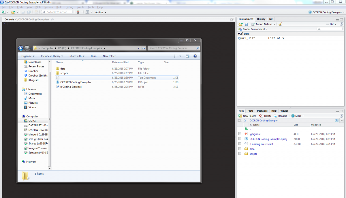
Whether you used the links on the DOI or used the script, the data files should be downloaded into the /data folder of your working directory. Now let’s load them into our R project in RStudio and look at the column headers. We will use the tidyverse method of loading csv files with read_csv(), which automatically converts data frames into tibbles.
# Load tidyverse packages
library(tidyverse)
# Load data
core_data <- read_csv("data/V1_Holmquist_2018_core_data.csv")
impact_data <- read_csv("data/V1_Holmquist_2018_impact_data.csv")
methods_data <- read_csv("data/V1_Holmquist_2018_methods_data.csv")
species_data <- read_csv("data/V1_Holmquist_2018_species_data.csv")
depthseries_data <- read_csv("data/V1_Holmquist_2018_depth_series_data.csv")
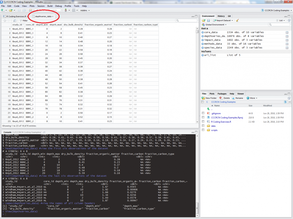
Tibbles are the tidyverse-preferred version of data frames, with superior display options and a simpler design. There are a variety of methods to quickly view our tibbles, such as the depthseries_data tibble:
# Display data
glimpse(depthseries_data) # View all column headers and a sample of observations
## Observations: 16,976
## Variables: 8
## $ study_id                <chr> "Boyd_2012", "Boyd_2012", "Boyd_2012",...
## $ core_id                 <chr> "BBRC_1", "BBRC_1", "BBRC_1", "BBRC_1"...
## $ depth_min               <int> 0, 4, 8, 12, 16, 20, 24, 28, 32, 36, 4...
## $ depth_max               <int> 2, 6, 10, 14, 18, 22, 26, 30, 34, 38, ...
## $ dry_bulk_density        <dbl> 0.28, 0.41, 0.40, 0.48, 0.54, 0.59, 0....
## $ fraction_organic_matter <dbl> 0.28, 0.23, 0.27, 0.20, 0.18, 0.16, 0....
## $ fraction_carbon         <dbl> NA, NA, NA, NA, NA, NA, NA, NA, NA, NA...
## $ fraction_carbon_type    <chr> NA, NA, NA, NA, NA, NA, NA, NA, NA, NA...
head(depthseries_data) # View the first six observations of the dataset
## # A tibble: 6 x 8
##   study_id  core_id depth_min depth_max dry_bulk_density fraction_organic~
##   <chr>     <chr>       <int>     <int>            <dbl>             <dbl>
## 1 Boyd_2012 BBRC_1          0         2             0.28              0.28
## 2 Boyd_2012 BBRC_1          4         6             0.41              0.23
## 3 Boyd_2012 BBRC_1          8        10             0.4               0.27
## 4 Boyd_2012 BBRC_1         12        14             0.48              0.2
## 5 Boyd_2012 BBRC_1         16        18             0.54              0.18
## 6 Boyd_2012 BBRC_1         20        22             0.59              0.16
## # ... with 2 more variables: fraction_carbon <dbl>,
## #   fraction_carbon_type <chr>
tail(depthseries_data) # View the last six observations of the dataset
## # A tibble: 6 x 8
##   study_id   core_id depth_min depth_max dry_bulk_density fraction_organi~
##   <chr>      <chr>       <int>     <int>            <dbl>            <dbl>
## 1 Windham_M~ GL              0         2             1.67          0.0545
## 2 Windham_M~ GL              8        10             1.92          0.00906
## 3 Windham_M~ HH              0         2             1.66          0.0270
## 4 Windham_M~ HH              8        10             1.34          0.0256
## 5 Windham_M~ HL              0         2             1.40          0.0579
## 6 Windham_M~ HL              8        10             1.87          0.00947
## # ... with 2 more variables: fraction_carbon <dbl>,
## #   fraction_carbon_type <chr>
names(depthseries_data) # View the names of all column headers
## [1] "study_id"                "core_id"
## [3] "depth_min"               "depth_max"
## [5] "dry_bulk_density"        "fraction_organic_matter"
## [7] "fraction_carbon"         "fraction_carbon_type"
The ability to quickly view your data in different ways will inform what manipulations are needed to be performed. Besides these commands, you can also click on an object in the “Environment” tab of RStudio:

Let’s take a quick look at the columns provided in the depthseries_data tibble (this metadata can be found online here, which is also linked on the dataset DOI):
| Column header | Meaning |
|---|---|
| study_id | Unique identified for the study made up of the first author’s family name, as well as the second author’s or ‘et al.’ |
| core_id | Unique identifier assiged to a core. |
| depth_min | Minimum depth of a sampling increment. |
| depth_max | Maximum depth of a sampling increment. |
| dry_bulk_density | Dry mass per unit volume of a soil sample. |
| fraction_organic_matter | Mass of organic matter relative to sample dry mass. |
| fraction_carbon | Mass of carbon relative to sample dry mass. |
| fraction_carbon_type | Code assigned to specify the type of measurement fraction_carbon represents. |
A lot of interesting types of data to work with here. But we can change what is included as well, by adding and removing columns.